Creating simulated data from a time series model in R

Introduction

This post discusses how to simulate data with similar statistical properties to a real financial time series. This is useful if you have a limited data source and you wish to generate more data in order to reduce the likelihood of overfitting. By generating multiple different time series all with similar statistical properties, you can optimise your trading strategy on thousands of datasets and choose the parameters which have the best results.
We will be using “AAPL” (Apple) for this example and will apply an ARIMA model on our data which will in turn be used to simulate some data.

The packages you will need are as follows:

install.packages("quantmod")
install.packages("forecast")

# If you already have them installed you can use the following:
library(quantmod)
library(forecast)

Download your data

In order to create a model we need some data, we will use Apples stock price which can be retrieved using the Quantmod package and the ticker for Apple which is AAPL, for your own project you can use any time series you wish.

getSymbols("AAPL")

## [1] "AAPL"

head(AAPL)

##            AAPL.Open AAPL.High AAPL.Low AAPL.Close AAPL.Volume AAPL.Adjusted
## 2007-01-03  12.32714  12.36857 11.70000   11.97143   309579900      10.36364
## 2007-01-04  12.00714  12.27857 11.97429   12.23714   211815100      10.59366
## 2007-01-05  12.25286  12.31428 12.05714   12.15000   208685400      10.51822
## 2007-01-08  12.28000  12.36143 12.18286   12.21000   199276700      10.57016
## 2007-01-09  12.35000  13.28286 12.16429   13.22429   837324600      11.44823
## 2007-01-10  13.53571  13.97143 13.35000   13.85714   738220000      11.99609

Model our data

We want to create a statistical model which has a good fit to our time series. We will achieve this by using the Arima function from the forecast package which will allow us to create a number of models and then choose the one that we deem to be the best fit. We will determine the best fit based on the AIC (Akaike Information Criterion) value, choosing the model with the smallest value.

Note that the snipper of code below has been taken from the Quantstart blog and tweaked to fit my project, the link to the full article containing the original code can be found in the references.

One of the key differences I have made is using the “Arima” function and supplying my data to the model without using the differenced log of the close price to transform it to stationary. Instead, I have used the argument lambda = 0 in my call to “Arima” which applies the Box-Cox transformation, this is also applied when simulating my data which has prevented the stock prices from dropping below 0, which wouldn’t occur in the marketplace.

# Before running our loop we create two objects which will contain the model with the best fit
final.aic <- Inf
final.order <- c(0,0,0)
# We use a loop to run through all the combinations of our ARMA model, where p represents the autoregressive part of our model and q represents our moving avaerage part
for (p in 0:5) for (q in 0:5) {
  if ( p == 0 && q == 0) {
    next
  }
  
  arimaFit = tryCatch( Arima(AAPL$AAPL.Close, order=c(p, 0, q), lambda = 0),
                       error=function( err ) FALSE,
                       warning=function( err ) FALSE )

  if( !is.logical( arimaFit ) ) {
    current.aic <- AIC(arimaFit)
    if (current.aic < final.aic) {
      final.aic <- current.aic
      final.order <- c(p, 0, q)
      final.arima <- Arima(AAPL$AAPL.Close, order=final.order, lambda = 0)
    }
  } else {
    next
  }
}

print(final.order)

## [1] 3 0 5

Simulating our data

The next step is to use the model that we chose above to generate simulated data which we can later use for our backtesting.

numberofobservations <- 1000 # can be any number you wish
set.seed(1) # this is purely for this demonstration, remove this if you are simulating data otherwise you'll get the same price series each time.
arima_simulation <- simulate(final.arima, nsim = numberofobservations, lambda = 0)
head(arima_simulation)

## Time Series:
## Start = 3377 
## End = 3382 
## Frequency = 1 
## [1] 316.9825 318.7347 313.1725 323.6708 325.7969 319.7002

Tidying and plotting the output

The periodicity of your data will determine the time between intervals that you enter in the “by =” argument below. For this example we are using the daily close of AAPL, therefore we use “day”, if we had minute data we would use “min”. The purpose of this step is to get our data into a suitable format before backtesting. The first object index_ts is a vector of dates which we will use as the index for our data when we create an xts object.

index_ts <- seq(from=as.POSIXlt("2010-01-01 00:00:00"), by = "day", length.out = numberofobservations)
xts_arima_simulation <- xts(arima_simulation, order.by = index_ts)
names(xts_arima_simulation) <- "close"

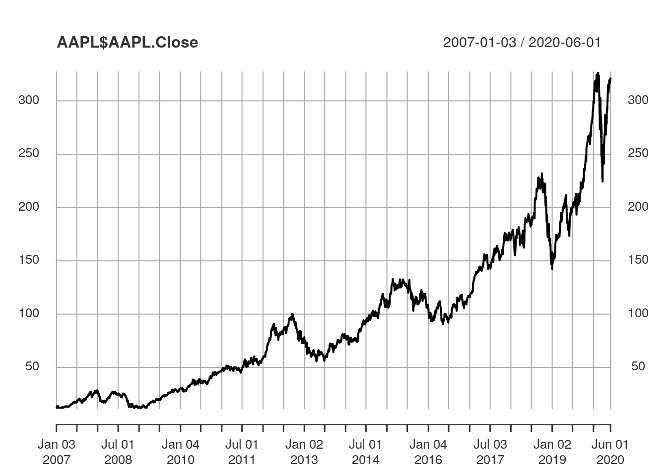
plot(AAPL$AAPL.Close, type="l")

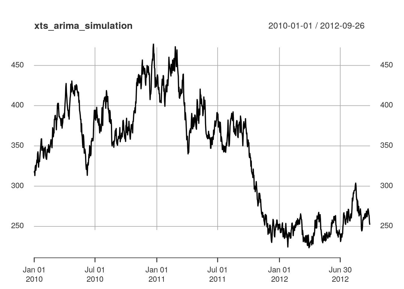
plot(xts_arima_simulation, type="l")

Conclusion

This has been a very quick demonstration on how to model a time series and generate some simulated data from it. If you would like some further information I have added a number of links in the section below.

References and reading material

Quantstart
The article linked below has some of the code for finding the best fitting ARIMA model.
https://www.quantstart.com/articles/ARIMA-GARCH-Trading-Strategy-on-the-SP500-Stock-Market-Index-Using-R/

Rob J Hyndman and George Athanasopoulos ,Forecasting: Principles and Practice
This is an online textbook written by the authors of the forecast package and contains information on ARIMA models in more detail amongst many other topics.
https://otexts.com/fpp2/arima.html